
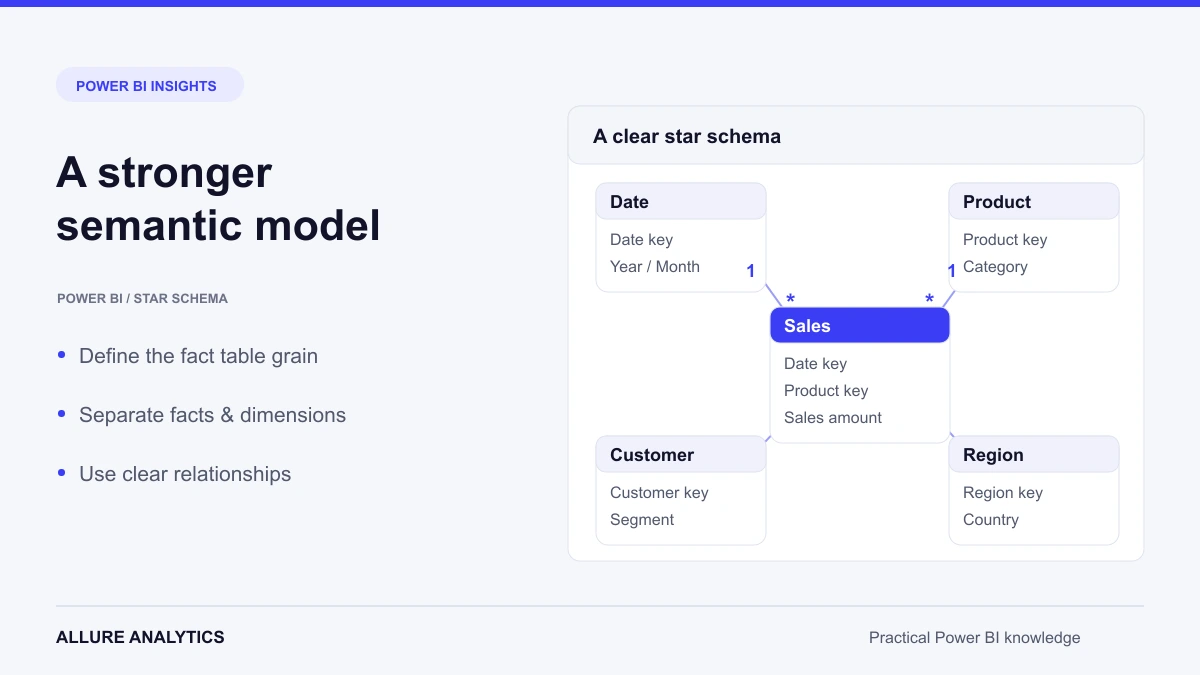
A well-designed Power BI semantic model makes reports easier to understand, validate and maintain. Clear table roles, consistent keys and predictable filter paths reduce unnecessary DAX complexity and support faster queries. This guide follows the original sequence of model-design and organization examples.
Control automatic relationship detection
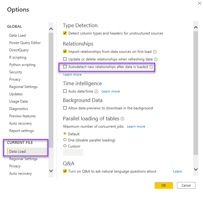
When a new table contains columns with names and values that resemble existing keys, automatic detection can propose relationships you did not intend. Review those suggestions before relying on the model. For a governed model, create and validate the required relationships deliberately.
Use a shared date table instead of unnecessary Auto date/time tables
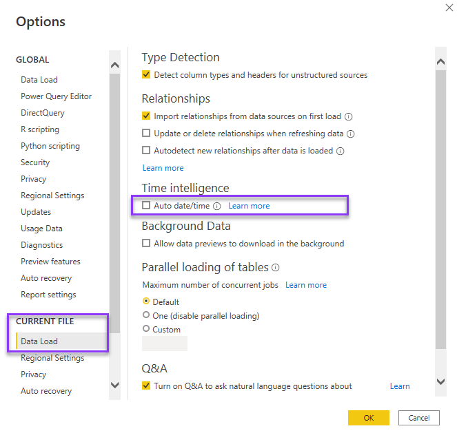
Auto date/time is convenient for simple exploration, but its hidden date tables are tied to individual date columns. A dedicated calendar dimension gives multiple fact tables a common definition of dates, fiscal periods and reporting attributes. Unnecessary automatic date tables can increase model size and refresh work. The calendar-table article shows how to create an explicit date dimension. here.
Choose visual cross-filtering intentionally
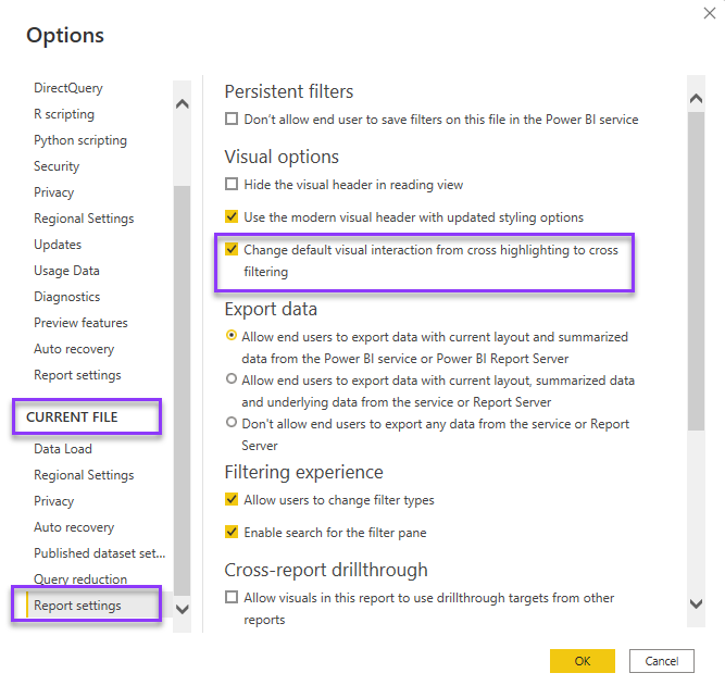
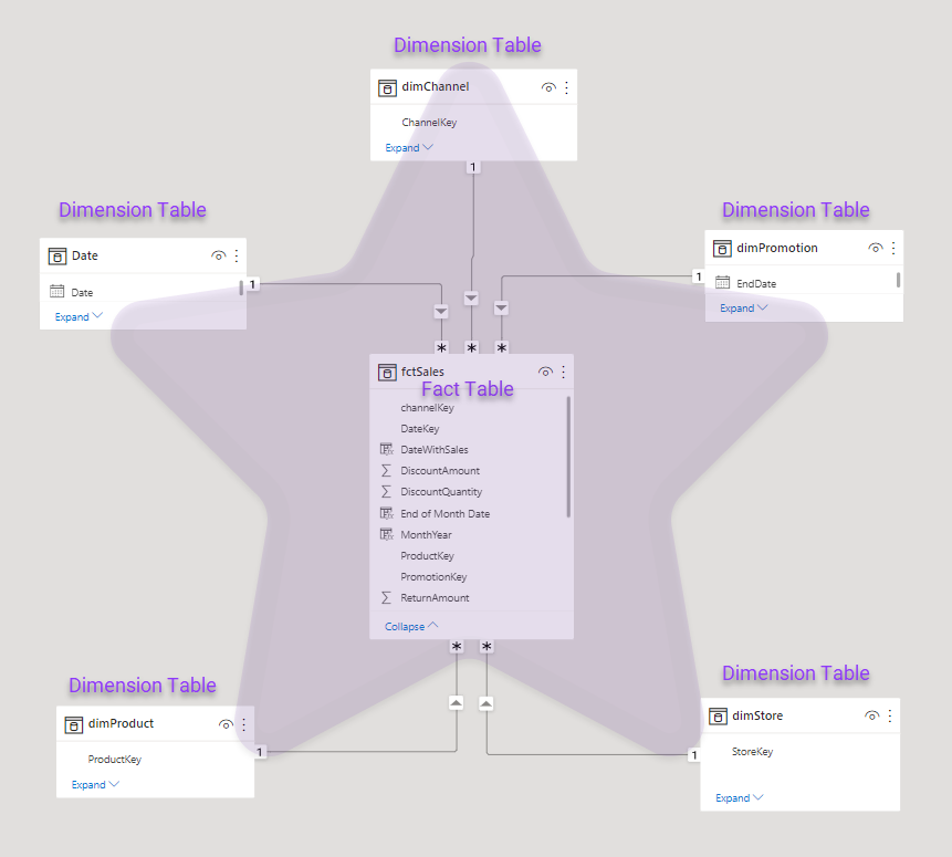
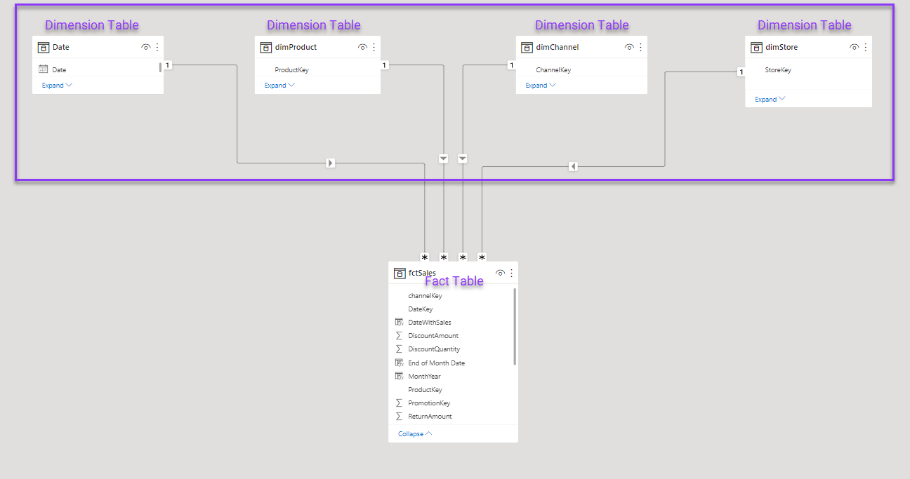
The Options screenshot illustrates the choice between cross-highlighting and cross-filtering for visual interactions. This behavior is separate from relationship filter direction. In Model view, arrange tables so their roles and filter paths are easy to follow. A star-shaped arrangement and a waterfall arrangement can describe the same star-schema relationships; the canvas layout is an organizational choice.
Star schema
Arrange the model as a star
One way to make the table roles visible is to arrange the model in a star shape.
- Place the fact table at the centre.
- Position the dimension or lookup tables around it.
In the illustration, fctSales is the central fact table and the surrounding dimensions supply filtering and descriptive attributes.
Arrange the model as a waterfall
A waterfall layout places dimension tables above the fact tables. It makes the intended dimension-to-fact filter direction easy to read.
- Use one row for dimensions and another for facts.
- Follow each dimension’s relationships down to the related facts.
- Keep relationship lines visible so unexpected connections are easier to spot.
Maintain the relationship definitions as deliberately as the visual arrangement.
- Review automatically generated relationships and remove those that are not required.
- Create the intended key relationships explicitly.
- Use Manage Relationships to inspect and maintain the complete relationship list.
Work with multiple fact tables
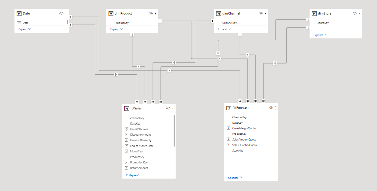
For the Actuals and Forecast scenario shown here, use shared dimensions rather than a direct fact-to-fact relationship.
Build the model around the grain of each fact table
Identify the Actuals and Forecast facts first. Define their granularity—for example, monthly forecast compared with more detailed actual transactions. Identify the common dimensions, such as Country and Date, and provide consistent foreign keys. Connect the facts through those dimensions using appropriate one-to-many relationships. A monthly forecast should not be treated as though it contains daily transaction detail.
Hide technical foreign keys
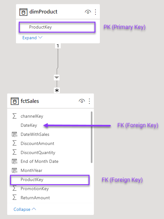
A primary key identifies a unique dimension row. A foreign key in a fact table points to that dimension row and may appear in many fact records. In the example, ProductKey is unique in dimProduct and can repeat in fctSales. Keep the relationship key available to the model, but hide technical foreign-key columns from report authors when they should use the dimension’s attributes instead.
Relationship cardinality
Cardinality describes whether the related columns contain unique or repeated values. The “one” side must contain unique values; the “many” side can contain duplicates.
Duplicate values introduced on the “one” side violate that relationship’s uniqueness requirement and can cause refresh to fail.
Power BI represents the four cardinality types with the following notation. One-to-one relationship guidance.
- One to many (1:*)
- Many to one (*:1)
- One to one (1:1)
- Many to many (*:*)
One-to-many and many-to-one describe the same relationship from opposite starting tables. Product to Sales is 1:* when ProductID is unique in Product and repeats in Sales. Reversing the table order gives Sales to Product as *:1.
One-to-one relationships
Both related columns must be unique in a one-to-one relationship. Check why the attributes are stored in separate tables and whether the design needs that separation. This relationship type is appropriate for some requirements, but it should be a deliberate modelling choice.
Many-to-many relationships
Both related columns can contain repeated values in a many-to-many relationship. This can support specific requirements, including facts stored above a dimension’s lowest grain. For example, a target at product-category level has a different grain from a product-level dimension. Power BI can infer cardinality from the available data or source profiling, but the inferred setting still needs review. Empty tables or temporarily unique sample data can produce a misleading inference. Any column used on the “one” side must remain unique when the full data is loaded.
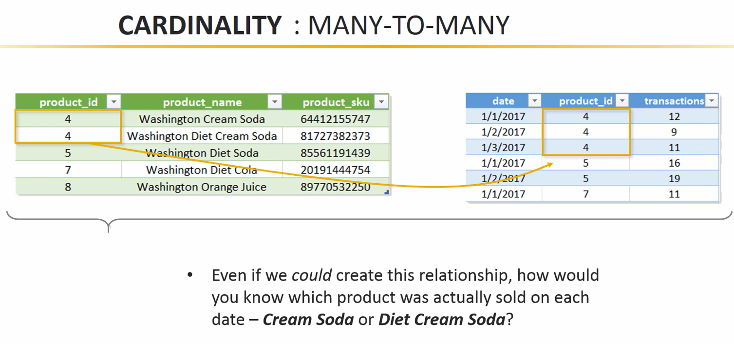
Use many-to-many relationships only when the grain and filter behaviour justify them. They are not a general substitute for resolving dimension keys or designing a bridge.
A conventional star schema normally uses one-to-many relationships from dimensions to facts.
Match the key-column data types
Use compatible data types for related keys and validate their values. A relationship between a numeric key and its text representation is not a reliable design.
The illustrated relationship uses the numeric ProductKey column.
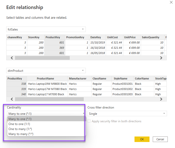
Many-to-one (*:1)
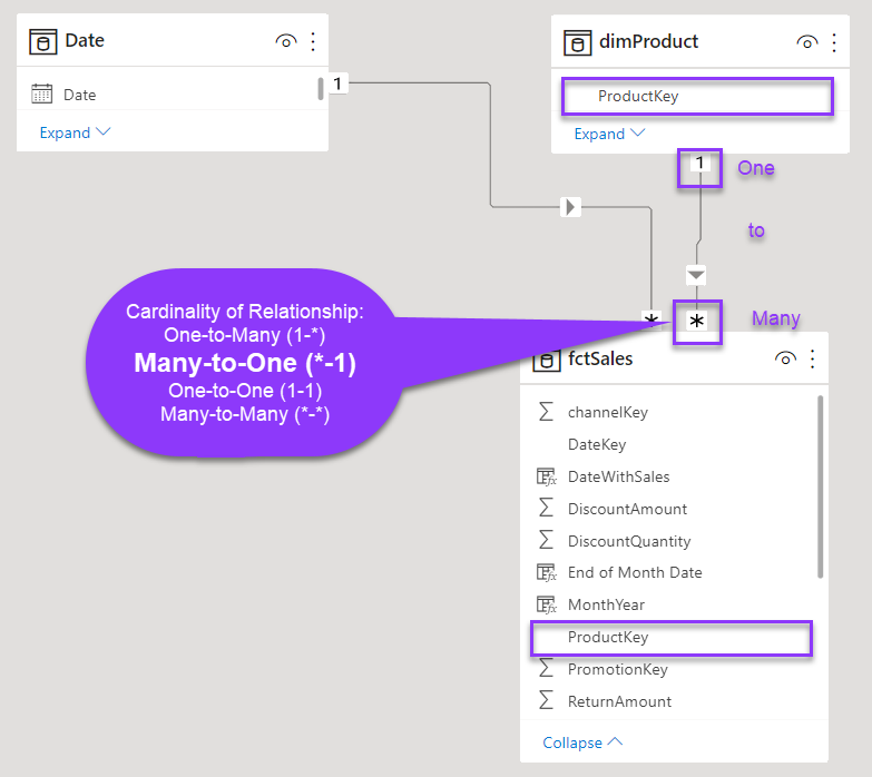
ProductKey contains unique values in dimProduct. The matching column in fctSales supplies the repeated foreign-key values.
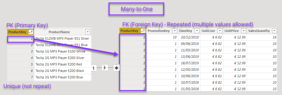
Relationship cross-filter direction
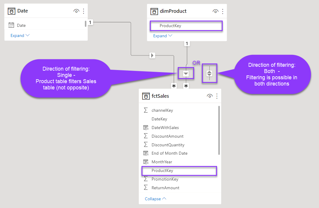
Cross-filter direction controls how filters propagate through a model relationship. The available settings depend on the relationship’s cardinality.
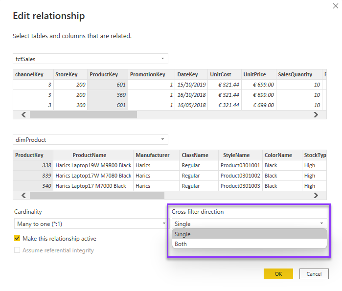
Use single-direction filtering from dimensions to facts as the default for this model. Bidirectional filtering can introduce ambiguous paths, extra query work and confusing slicer behaviour. Introduce it only for a specific, tested requirement; a snowflake layout alone is not a reason to enable it. Bidirectional-filter guidance.
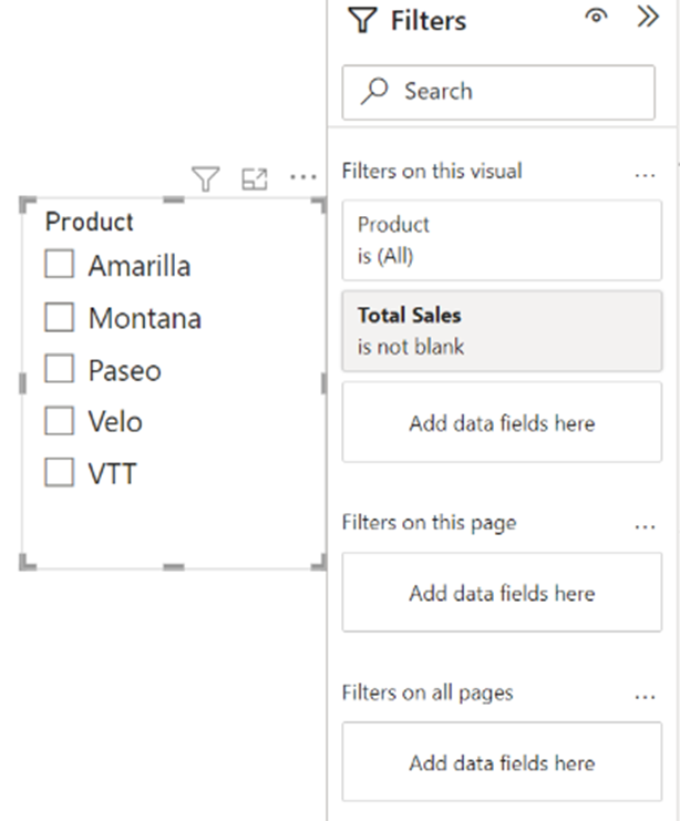
If the requirement is simply to show slicer items that have data, consider a visual-level “is not blank” filter based on an appropriate measure. Configure that behaviour for each relevant slicer rather than adding bidirectional relationships throughout the model.
Active and inactive relationships
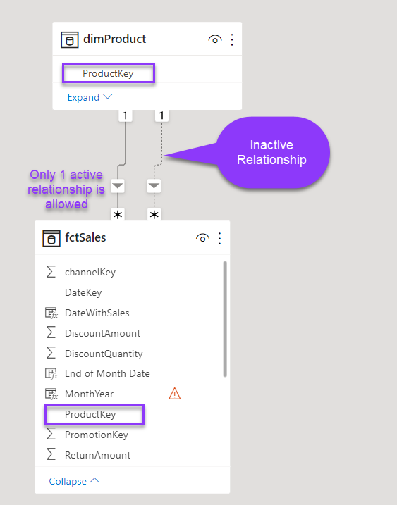
An inactive relationship is shown as a dashed line. Avoid competing active filter paths between the same tables.
A model can retain alternative relationships while using only the intended active filter path. USERELATIONSHIP activates a specified existing relationship for a calculation. A common example is a role-playing Date dimension: sales may contain Order Date, Ship Date and Delivery Date, with a different date role needed by each measure.
Original typographic quotes are retained. “Copy straight quotes” changes only those quote characters when pasting into an editor that requires standard DAX quotation marks.
Orders Shipped =
CALCULATE(
    COUNTROWS(fctSales)
    ,USERELATIONSHIP(‘Date’[Date], fctSales[ShipDate])
)
Create a dedicated measures table
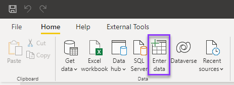
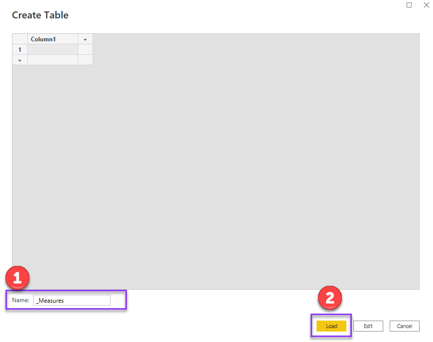
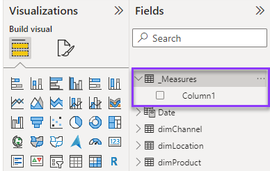
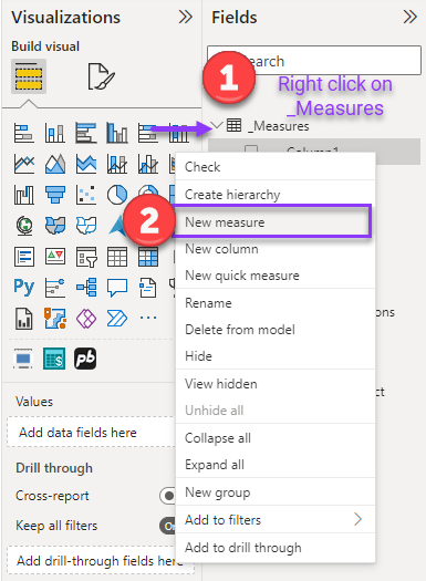
Keep measures easy to find by assigning them to a dedicated measures table or a clearly organized set of tables. The original walkthrough creates a small table and then uses it as the home for measures.
1. Add a new table
2. Name the table and load it
3. Confirm that the table appears in the model
4. Assign a measure to the table
Create the first measure using the source expression below.
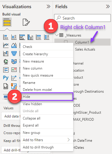
Sales Actuals = SUM(fctSales[SalesAmount])5. Hide the placeholder Column1
Format DAX for readability
Use line breaks and indentation to make nested expressions easier to read. Formatting should clarify the expression without changing its calculation.
DAX Studio and DAX Formatter can also help format expressions. Review the output before replacing a measure.
Use a consistent naming convention, including CamelCase for hidden technical columns where that is your model standard.
1. Add line breaks
Sales Actuals =
SUM(fctSales[SalesAmount])2. Indent nested expressions
Original typographic quotes are retained. “Copy straight quotes” changes only those quote characters when pasting into an editor that requires standard DAX quotation marks.
Sales Actuals Red =
CALCULATE(
 SUM(fctSales[SalesAmount]),
    dimProduct[ColorName] = “Red”
)
3. Add comments to explain intent. Use // or — for a single-line comment and /* … */ for a block comment.
Original typographic quotes are retained. “Copy straight quotes” changes only those quote characters when pasting into an editor that requires standard DAX quotation marks.
Sales Actuals Red =
//Calculate only Red products
CALCULATE(
SUM(fctSales[SalesAmount]),
    dimProduct[ColorName] = “Red”
)
The archived expression ends before the outer CALCULATE is closed. The original is preserved; complete the syntax before executing this example.
Original typographic quotes are retained. “Copy straight quotes” changes only those quote characters when pasting into an editor that requires standard DAX quotation marks.
Sales Actuals =
CALCULATE(
SUM(fctSales[SalesAmount])
/*
CALCULATE(
SUM(fctSales[SalesAmount]),
    dimProduct[ColorName] = “Red”
)
*/
Use variables to name intermediate results and avoid unnecessary repeated evaluation within the expression. A variable is evaluated in the context where it is defined; moving a calculation into a variable can therefore affect context-sensitive logic.
Choose descriptive variable names, such as _TotalSales.
The original sample filters ProductName to “Red”. If the requirement is red-coloured products, check that the intended attribute is ColorName before adapting it.
Original typographic quotes are retained. “Copy straight quotes” changes only those quote characters when pasting into an editor that requires standard DAX quotation marks.
Sales % Red =
VAR _RedProducts = CALCULATE(SUM(fctSales[SalesAmount]), dimProduct[ProductName] = “Red”)
VAR _TotalActuals = SUM(fctSales[SalesAmount])
RETURN
    DIVIDE(_RedProducts, _TotalActuals)
Organize measures with display folders
As the number of measures grows, display folders make the model easier to browse. Use Model view to select measures and assign the required Display folder property.
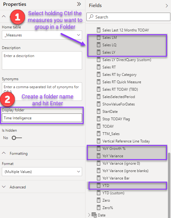
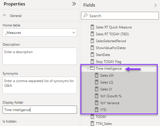
The folder appears under the measures’ home table. Continue assigning measures to the appropriate folders as the model develops.
Create a Date dimension
Use a shared Date dimension for the model’s date filtering and classic time-intelligence calculations. The calendar-table article provides the construction steps and source code. here.
Review calculated columns that use RELATED. Keep required row-level attributes, and remove redundant stored values where a better model design can supply the same reporting need.
Use descriptive, consistent names for calculated columns, measures and variables. The original naming examples are TotalSales, Sales, Fact_Sales, fctSales, DimProduct and _LastMonth.
Use a consistent function-casing style in DAX. IntelliSense can help apply uppercase function names such as SUM and CALCULATE. The archived example below is retained as written.
Sales Actuals =
sum(fctSales[SalesAmount])
Apply consistent numeric, percentage and date formats to the measures and columns exposed to report authors.
Use disconnected tables for parameter selections
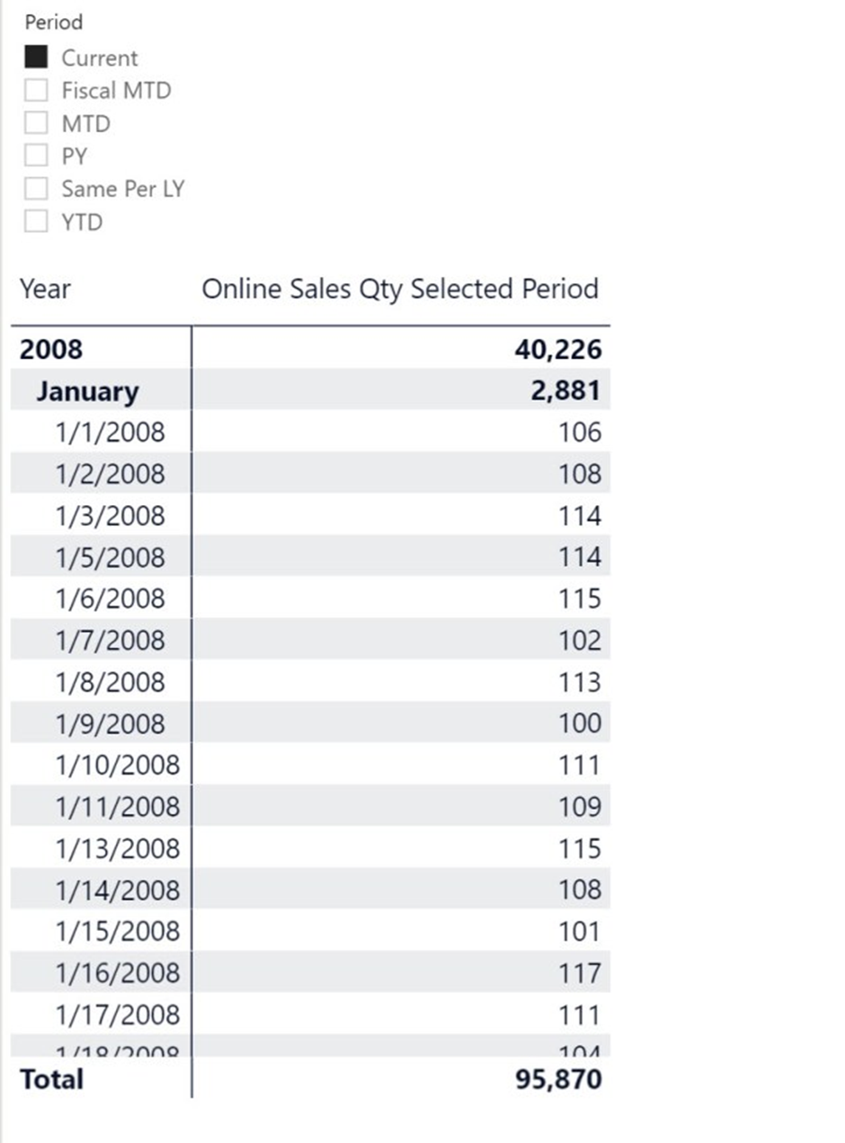
A disconnected table can capture a user’s selection without propagating a relationship filter. A measure then interprets that choice, for example to switch between current values, MTD and YTD calculations.
Field Parameters can address some report-switching requirements too. Choose the technique that fits the model and the behaviour you need.
The example uses Enter Data to create a Period column containing Current, MTD, YTD, Same Per LY and PY. The model contains Store Sales Qty measures for those time selections. Store Sales Qty sums Quantity, while the MTD measure restricts the calculation to the selected month-to-date period. Store Sales Qty Selected Period uses the disconnected selection to return the chosen measure. The screenshots below show the selector and the original expression.
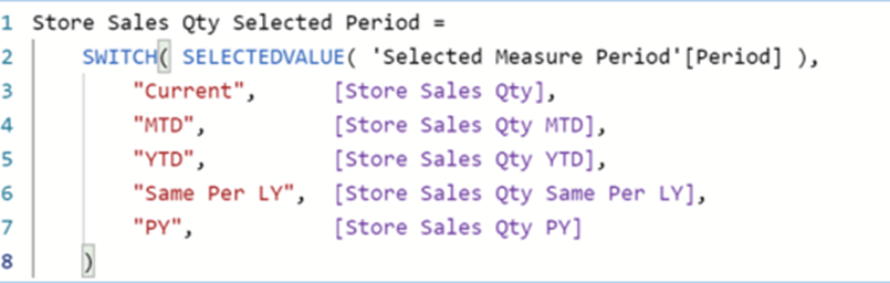
Expression transcribed from the original illustration
Store Sales Qty Selected Period =
    SWITCH( SELECTEDVALUE( 'Selected Measure Period'[Period] ),
        "Current",     [Store Sales Qty],
        "MTD",         [Store Sales Qty MTD],
        "YTD",         [Store Sales Qty YTD],
        "Same Per LY", [Store Sales Qty Same Per LY],
        "PY",          [Store Sales Qty PY]
    )
Model-review checklist. The original Best Practice Analyzer-style rules are retained below in their original category order. Treat them as review prompts rather than universal bans: some require additional scripts or depend on model requirements. The original asterisk markers are retained. DIVIDE. IFERROR. TREATAS. INTERSECT. RELATED.
- Use DIVIDE where the denominator can be zero or BLANK.
- Review IFERROR usage and handle the intended condition explicitly where appropriate.
- Qualify column references with their table names.
- Reference measures without a table prefix.
- Review measures that only alias another measure; retain aliases when they serve an intentional reporting or metadata purpose.
- Review duplicate measure definitions and centralize common logic where appropriate.
- Consider TREATAS for an explicitly designed virtual relationship; validate its filter semantics rather than replacing INTERSECT mechanically.
Error prevention
- Check that data columns have valid source-column mappings.
- Check that calculated columns contain valid expressions.
Formatting
- Assign data categories where they describe the column’s meaning.
- Set technical numeric attributes to Do not summarize where aggregation would be misleading.
- Apply the model’s chosen capitalization convention consistently.
- Hide technical fact-table columns that report authors should not use directly.
- Hide technical foreign keys from report authors.
- Identify and validate dimension primary keys.
- Sort month-name columns by the intended month number.
- Remove accidental leading or trailing spaces from object names.
- Use a consistent percentage format and precision suited to the measure.
- Give flag columns meaningful Yes/No display values where appropriate.
- Set suitable date-column formats.
- Set suitable month-column formats.
- Define format strings for exposed measures.
- Prefer appropriate, consistent key types; integer keys are often useful, but are not mandatory for every relationship.
- Format whole-number measures with suitable grouping and precision.
Maintenance
- Review tables without relationships and confirm whether each is intentionally disconnected.
- Add useful descriptions to model objects.
- Remove data sources that no partition uses.
- Review roles without assigned members; retain roles that are provisioned elsewhere intentionally.
- Remove unnecessary columns.
- Remove unnecessary measures.
Naming conventions
- Apply CamelCase consistently where used for hidden columns.
- For single-partition tables, use a clear partition name aligned with the table name.
- Use object names that remain readable and work well with your tooling.
Performance
- Review bidirectional filters on high-cardinality columns. *
- Minimize unnecessary bidirectional and many-to-many relationships.
- Prefer clear star-schema relationships; review whether snowflaking adds avoidable complexity.
- Choose numeric types and precision deliberately; do not convert every floating-point value indiscriminately.
- Consider partitions for large tables when the deployment and refresh strategy support them. *
- Keep row-level security logic focused and validate its performance.
- Review the direction of many-to-many filter propagation carefully.
- Push suitable transformations upstream or preserve query folding where possible.
- Provide a shared Date dimension for the model’s reporting requirements.
- For DirectQuery models, review whether aggregations fit the workload.
- Reduce unnecessary calculated columns.
- Review calculated columns using RELATED for redundant storage.
- Review whether calculated tables are needed.
- Reduce unnecessary long, high-cardinality text columns. **
- Remove unused automatic date tables when an explicit date dimension provides the required behaviour.
- Remove redundant columns from related tables.
- Review IsAvailableInMdx for technical, non-attribute columns where your tools support that setting.
- Separate date and time when their cardinality and reporting use justify it. ***
- Mark date tables when the classic time-intelligence pattern requires it.
- Unpivot repeated month columns when that produces the appropriate analytical grain.