
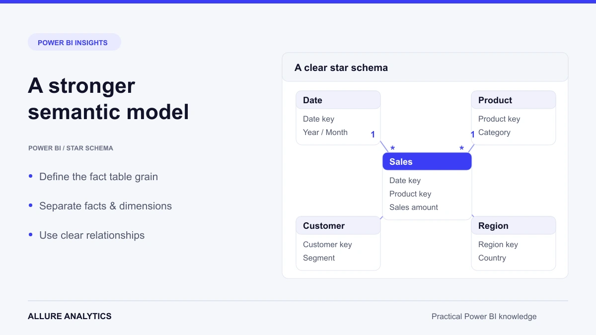
A well-designed semantic model makes the same business question return the same answer, wherever it appears in the report. Begin with the meaning and grain of the data, then build relationships and measures around that contract.
Separate facts from dimensions
A fact table records events or measurements: sales lines, production observations or monthly forecasts. A dimension describes the entities used to filter and group them: products, customers, machines or dates. State what one row represents in every fact table before designing relationships.
A star schema connects dimensions to facts with clear filtering paths. Rearranging tables into a waterfall layout can improve readability in Model view, but the diagram’s position does not change the relationships or their behaviour. Microsoft star-schema guidance.
Use shared dimensions across multiple facts
Sales actuals and forecasts can be analysed together through shared Date and Product dimensions. Avoid a direct fact-to-fact relationship as the default solution. When the facts have different grains, document the level at which their values can be compared.
For example, a monthly forecast and daily sales support a monthly comparison. A daily comparison needs an agreed allocation rule for the forecast. A relationship alone cannot create that business definition.
Check keys, cardinality and filter direction
- The key on the one side must be unique. Investigate duplicates before creating the relationship.
- Use compatible data types on both sides of a relationship.
- A fact usually contains repeated foreign keys on the many side.
- Single-direction filtering from dimension to fact is a useful default.
- Many-to-many and bidirectional relationships can be appropriate, but need a clear reason and tests for ambiguous filtering.
Hide technical keys from report authors when they are not useful for analysis. Keep business-facing names clear, and retain the keys and relationship documentation for model maintenance.
Model date roles explicitly
An order can have an order date and a ship date. One Date dimension can use an active order-date relationship and an inactive ship-date relationship, with a measure that activates the latter when needed. Separate role-playing date dimensions are another option when users need independent date slicers.
DAX
Orders = COUNTROWS ( Sales )

Orders by Ship Date =
CALCULATE (
    [Orders],
    USERELATIONSHIP ( 'Date'[Date], Sales[ShipDate] )
)
USERELATIONSHIP uses an existing relationship for the calculation. Validate the competing date paths and the current filter context. Relationship restrictions apply to specific table pairs and filtering paths; they do not mean that a whole model can have only one active relationship.
Take control of automatic settings
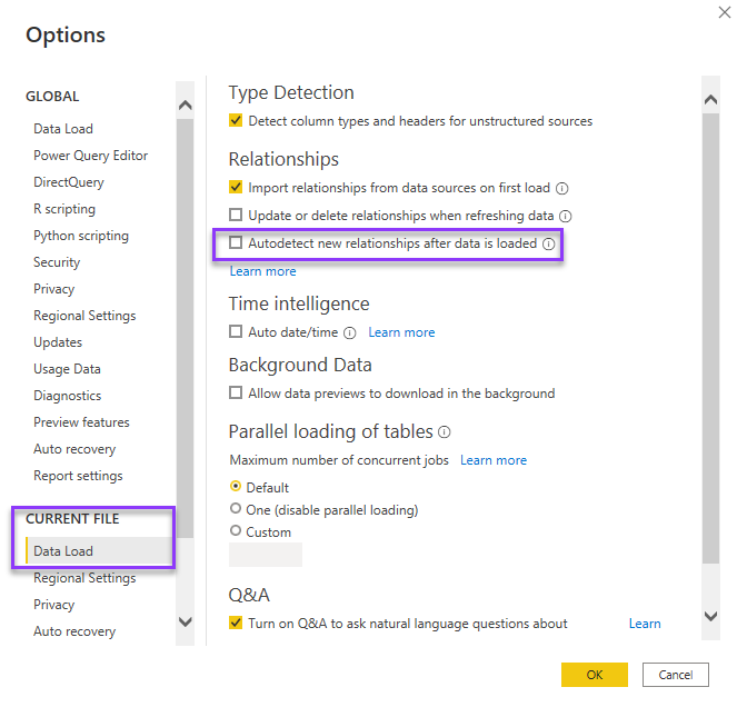
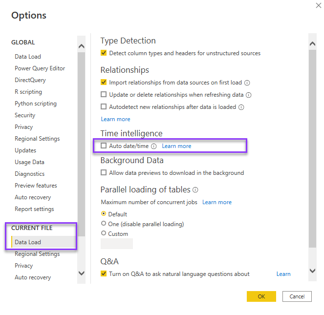
Automatic relationship detection and auto date/time can speed up exploration. In a maintained model, review what they create and replace convenience structures where a shared model definition is needed. Do not delete valid relationships simply because they were detected automatically.
Organise measures around business definitions
Use explicit measures for reusable business logic. Display folders and a dedicated measures table make a large model easier to navigate. Give percentages, currency and counts suitable formats, and add descriptions for calculations with important assumptions.
DAX
Gross Profit = [Sales Amount] - [Cost of Sales]

Gross Margin % =
VAR Revenue = [Sales Amount]
VAR Profit = [Gross Profit]
RETURN DIVIDE ( Profit, Revenue )
Variables improve readability and can avoid repeating an expression in the same evaluation context. They are evaluated where they are defined, so moving an expression into a variable can change a calculation if you later expect it to respond to a modified context.
Choose interactions and selectors deliberately
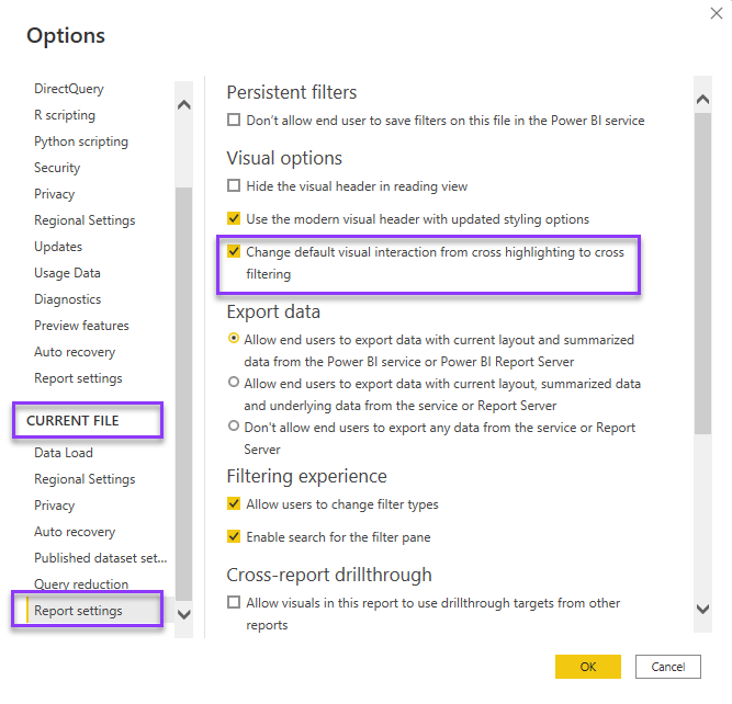
Cross-highlighting shows a selected contribution alongside the full total. Cross-filtering narrows the receiving visual. Choose the interaction that fits the reporting task and keep the selected context clear.
A disconnected selector table with SELECTEDVALUE and SWITCH is useful for a controlled business choice. Field parameters solve a related but different need: allowing readers to choose fields or measures displayed in a visual. Use the mechanism that matches the user’s task.
Balance accuracy, size and maintainability
- Choose data types for the precision the business needs; floating-point and fixed-decimal types have different uses.
- Remove unused columns and unnecessary history within the approved reporting scope.
- Plan refresh and partitioning around operational needs, rather than a single row-count rule.
- Test relationships and measures with totals, missing members and unusual filter combinations.
- Use model-analysis rules as review guidance, and document justified exceptions.
A clean model is a practical asset: it gives report authors a dependable vocabulary and gives future maintainers a clear path through the logic.
Complete DAX and Power Query reference
The following reference retains every substantive code example from the supplied article, including alternative approaches and examples that demonstrate a problem. Table names and historical date ranges are preserved. Compare these alternatives with the updated guidance above before adapting them to your model.
Orders Shipped
The archived code contains typographic quotation marks. Replace them with straight single or double quotes before using the expression in the DAX editor.
DAX
Orders Shipped =
CALCULATE(
    COUNTROWS(fctSales)
    ,USERELATIONSHIP(‘Date’[Date], fctSales[ShipDate])
)
Sales Actuals
DAX
Sales Actuals =
SUM(fctSales[SalesAmount])
Sales Actuals
DAX
Sales Actuals =
SUM(fctSales[SalesAmount])Sales Actuals Red
The archived code contains typographic quotation marks. Replace them with straight single or double quotes before using the expression in the DAX editor.
DAX
Sales Actuals Red =
CALCULATE(
 SUM(fctSales[SalesAmount]),
    dimProduct[ColorName] = “Red”
)
Sales Actuals Red
The archived code contains typographic quotation marks. Replace them with straight single or double quotes before using the expression in the DAX editor.
DAX
Sales Actuals Red =
//Calculate only Red products
CALCULATE(
SUM(fctSales[SalesAmount]),
    dimProduct[ColorName] = “Red”
)
Sales Actuals
The archived code contains typographic quotation marks. Replace them with straight single or double quotes before using the expression in the DAX editor. The archived example has unbalanced parentheses. It is retained for completeness; correct the syntax before execution.
DAX
Sales Actuals =
CALCULATE(
SUM(fctSales[SalesAmount])
/*
CALCULATE(
SUM(fctSales[SalesAmount]),
    dimProduct[ColorName] = “Red”
)
*/
Sales % Red
The archived code contains typographic quotation marks. Replace them with straight single or double quotes before using the expression in the DAX editor. Review the product filter in this source example: a colour calculation should filter the colour attribute, and the variable name used in RETURN must match its declaration.
DAX
Sales % Red =
VAR _RedProducts = CALCULATE(SUM(fctSales[SalesAmount]), dimProduct[ProductName] = “Red”)
VAR _TotalActuals = SUM(fctSales[SalesAmount])
RETURN
    DIVIDE(_RedProducts, _TotalActuals)
Full source narrative and setup notes
Read every original instruction and explanation
This reference preserves the original article’s prose, setup steps and small inline expressions. Historical interface labels and recommendations are retained for comparison with the updated guidance above.
I wanted to highlight in this post some of my best practice tips for Power BI data modeling.
Data modeling is one of the foundations of your Power BI reports, so it’s important to set it up correctly. It’s crucial to create a well-developed data model to help you fully communicate your organization’s information. Data modelling helps you optimize your tables and columns. Doing it right will save you so much time.
These tips and best practices will help you create a more organized model, making it easier for you to understand the relationships in your data set. Once you’ve fully grasped how to set up data models, you can easily create intuitive and meaningful Power BI reports.
Benefits of using a Good Data Model:
• Increased report performance • Less complex DAX to be used and accurate results • Queries will load faster
Disable Autodetect new relationships option
If you add a new table to the model that has field names (and values) matching with other tables in the model, then Power BI automatically creates a relationship between each of the existing tables and the new table, and this can be sometimes too many new relationships.
This can lead to an unexpected relationships and would cause data issues.
Disable Auto date/time option
The main purposes of the auto date/time are to support convenient time intelligence reporting based on the date columns loaded into the data model.
Instead of using this date hierarchy which is not complete, just create a Date Calendar Table. How to create a Date Calendar Table can be found here
For each date column that generates a hidden auto date/time table, it will result in an increased model size and also extend the data refresh time.
Enable Visual cross-filtering
When setting up your data model, start by organizing your tables. One of the best ways to do this is by using the Waterfall technique (layout). Another way to do this effectively is by using the Star Schema approach.
The Layout method – Waterfall or stacked around the fact table(s) as a STAR model, does not matter as long as you understand it
My personal preference is the Waterfall layout, as you can visualize how the data will be filtered (also called “Lookup” Layout)
STAR SCHEMA
The *STAR* Layout
One of the ways is by using the Star Layout
Fact table at the center of the star
Dimension (Lookup) tables at the end points of the star
The Waterfall Layout
The second approach and layout for data modelling in Power BI is called the Waterfall technique. You set up your Dimension Tables at the top and the Fact Tables at the bottom.
Here are some of the benefits of this approach:
Arranges tables in rows (Dimension tables in the first row, Fact tables in the second row).
Easy to visualize the dimensions “falling” to the Fact table.
Displays all relationships and makes it easier to see errors.
When using this layout, you need to remember these details:
Delete any relationships autogenerated by Power BI.
Manually create all relationships.
Use the “Manage Relationships” dialogue to maintain relationships.
Handling Multiple Fact Tables
So maybe you are thinking of having a multi-fact table model, how do you go about doing this?
You will need to do the following. I have provided an example from the few points above.
1. Identify the two fact tables — Actuals & Forecast
2. Agree on the granularity — Monthly, with the ability to drill
3. Identify the common dimensions — Country and Dates (create a FK)
4. Link the dimensions — Only Many to one (One to Many) cardinality
Hide Foreign Key (FK)
What is a foreign key? In your data model, you create relationships between a Primary Key (PK) and a Foreign Key (FK). An example of that is demonstrated below.
In the dimProduct table, you have a list of all products of your company. Each product is listed exactly one time, so you have unique values. This is your Primary Key.
In the fctSales table, a product could have multiple sales or no sales at all. This is the Foreign Key.
The Foreign Key should not be used in the Report View and should therefore be hidden (right click on it and select Hide in report view or click on the eye icon to hide).
RELATIONSHIP CARDINALITY
Each model relationship is defined by a cardinality type. There are four cardinality type options, representing the data characteristics of the “from” and “to” related columns. The “one” side means the column contains unique values; the “many” side means the column can contain duplicate values.
The four options, together with their shorthand notations, are described in the following bulleted list:
One to many (1:*)
Many to one (*:1)
One to one (1:1)
Many to many (*:*)
The one-to-many and many-to-one cardinality options are essentially the same, and they’re also the most common cardinality types.
When configuring a one-to-many or many-to-one relationship, you’ll choose the one that matches the order in which you related the columns. Consider how you would configure the relationship from the Product table to the Sales table by using the ProductID column found in each table. The cardinality type would be one-to-many, as the ProductID column in the Product table contains unique values. If you related the tables in the reverse direction, Sales to Product, then the cardinality would be many-to-one.
Please check the below example of Many to one cardinality relationship.
One-to-one cardinality
A one-to-one relationship means both columns contain unique values. This cardinality type isn’t common, and it likely represents a suboptimal model design because of the storage of redundant data.
For more information on using this cardinality type, see One-to-one relationship guidance.
Many-to-many cardinality
A many-to-many relationship means both columns can contain duplicate values. This cardinality type is infrequently used. It’s typically useful when designing complex model requirements. You can use it to relate many-to-many facts or to relate higher grain facts. For example, when sales target facts are stored at product category level and the product dimension table is stored at product level.
When you create a relationship in Power BI Desktop, the designer automatically detects and sets the cardinality type. Power BI Desktop queries the model to know which columns contain unique values. For import models, it uses internal storage statistics; for DirectQuery models it sends profiling queries to the data source. Sometimes, however, Power BI Desktop can get it wrong. It can get it wrong when tables are yet to be loaded with data, or because columns that you expect to contain duplicate values currently contain unique values. In either case, you can update the cardinality type as long as any “one” side columns contain unique values (or the table is yet to be loaded with rows of data).
Data type should match
The below example the relationship is based on ProductKey which is numeric (number)
The ProductKey column in the dimProduct table contains unique values.
Cross filter direction
Each model relationship is defined with a cross filter direction. Your setting determines the direction(s) that filters will propagate. The possible cross filter options are dependent on the cardinality type.
Alternatively, to avoid using bi-directional relationships, you can add a filter to the slicer visual to exclude items that are blank. It is worth noting that you would need to do this for each visual that uses fields across dimension tables.
Active or Inactive Relationship?
There can only be one active filter propagation path between two model tables. However, it’s possible to introduce additional relationship paths, though you must set these relationships as inactive. Inactive relationships can only be made active during the evaluation of a model calculation. It’ is achieved by using the USERELATIONSHIP DAX function.
An example of using Inactive relationships is so called Role Playing Dimensions
A role-playing dimension is a dimension that can filter related facts differently. For example, at Adventure Works, the date dimension table has three relationships to the reseller sales facts. The same dimension table can be used to filter the facts by order date, ship date, or delivery date.
Create Measure Table
In order to have a well structured report and keep your data model organized, it’s best to organize measures in separate tables. See below how to create dedicated Measures Tables:
1. Add a new table
2. Name the table and load it to the report
3. The new table has been added to the report
4. Allocate a new measure to this table
5. Hide Column1
Format your measures
DAX measures can become quite complex. To still be able to read complex DAX functions, you should consider adding some formatting to the formula in order to increase readability.
1. Add line breaks. Use Shift + Enter to add a line break (Alt + Enter)
2. Indent to create a structure. Use Tab key to indent
3. Add comments. For more complex DAX measure, you can add comments to explain what the measure is calculating. * For short use // or — * For multiple code lines you can use block comment /* your dax code */
Try to use good variable names like _TotalSales
Organize your measures in folders
Often, you end up having a big number of measures in a report. To still have the overview, you can organize measures in folders. To create and manage folders, you need to go to the Model view.
The newly created measure folder will appear in your model.
Once a folder has been created, you can also use drag and drop to move measures in between folders.
Create Date Dimension Table
Date table will not be discussed in this post. How to create a date dimension can be found here
Disconnected tables and their purpose
Disconnected tables are useful in a variety of ways, allowing a user to select a value that drives the behavior of a dynamic measure, or by grouping values and performing some kind of dynamic calculation.
Typical use of disconnected tables is toggle slicers, i.e. MTD/YTD
This table was created using the Enter Data feature and includes only one column named Period, which includes the following values:
Current MTD YTD Same Per LY PY
The purpose of this post is to demonstrate effective data modeling and not DAX fundamentals but one cannot exist without the other. For our purposes, my model in this example contains five measures that calculate the Store Sales Qty with different time series variations. The Store Sales Qty measure simply returns the Sum of the Quantity field and the Store Sales Qty MTD calculates the month-to-date value for a given date. I’ve created another measure named Store Sales Qty Selected Period which is shown below. When a value in this table is selected, this measure returns the results of one of the other measures.
The Rules
Now, let’s see the Best Practice Rules. As you can see below, the rules are segmented into categories. Some rules are more aesthetic-oriented while others are more focused on performance optimization. Note that there are several rules which require running an additional script (each is marked with an asterisk below).
DAX Expressions
Use the DIVIDE function for division
Avoid using the IFERROR function
Column references should be fully qualified
Measure references should be unqualified
Measures should not be direct references of other measures
No two measures should have the same definition
Use the TREATAS function instead of INTERSECT for virtual relationships
Error Prevention
Data columns must have a source column
Calculated columns must have an expression
Formatting
Add data category for columns
Do not summarize numeric columns
First letter of objects must be capitalized
Hide fact table columns
Hide foreign keys
Mark primary keys
Month (as a string) must be sorted
Objects should not start or end with a space
Percentages should be formatted with thousands separators and one decimal
Format flag columns as Yes/No value strings
Provide format string for “Date” columns
Provide format string for “Month” columns
Provide format string for measures
Relationship columns should be of integer data type
Whole numbers should be formatted with thousands separators and no decimals
Maintenance
Ensure tables have relationships
Objects with no description
Remove data sources not referenced by any partitions
Remove roles with no members
Remove unnecessary columns
Remove unnecessary measures
Naming Conventions
Use CamelCase for hidden columns
Partition name should match table name for single partition tables
Object names must not contain special characters
Performance
Avoid bi-directional relationships against high-cardinality columns *
Avoid excessive bi-directional or many-to-many relationships
Avoid snowflake schema architecture
Do not use floating point data types
Large tables should be partitioned *
Limit row level security (RLS) logic
Many-to-many relationships should be single direction
Minimize Power Query transformations
Model should have a date table
Model using Direct Query and no aggregations
Reduce number of calculated columns
Reduce usage of calculated columns that use the RELATED function
Reduce usage of calculated tables
Reduce usage of long-length columns with high cardinality **
Remove auto-date table
Remove redundant columns in related tables
Set IsAvailableInMdx to false on non-attribute columns
Split date and time ***
Date/calendar tables should be marked as a date table
Unpivot pivoted (month) data